This is a very short survey of how typical ODE solvers work. In particular, we describe one-step, Runge-Kutta solvers, which are the basis of most of the solvers in EJS. The text includes references to the parameters you can customize in the EJS ODE editor and its Advanced dialog.
Discretization
Suppose t is the current time. To provide the approximated solution of the ODE at a future time, an ODE solver discretizes the time axis and seeks to find a solution at t+dt, where dt is a convenient, usually small value. (For what small means, read below.) How the solver computes this approximation depends on its type. That is, an Euler solver will do it differently to the classic Runge-Kutta 4th-order solver.
A one-step solver uses only the current value of the state variables as the starting point to approximate the future state. Multistep solvers use also past values of the state. All solvers in EJS are one-step.
Order of an algorithm
The order of an algorithm indicates how good its approximation to the solution is. Thus, for instance, a 4th-order algorithm provides an approximation at t+dt that has an error of the size of dt5. (Yes, 5=4+1.) This means that after steeping repeatedly the algorithm, you get a 4th-order error in the solution per unit of time. On the other hand, this also implies that, if dt is small enough, the approximation converges to the real solution at t+dt.
Choosing the order of the solver is an important decision. No single solver is always THE right choice. A simple rule of thumb is the following: the higher the order of an algorithm, the more accurate it is. But also, the more computationally intensive. For standard problems, 4th or 5th-order methods are a safe bet. For simpler problems, a 2nd or 3rd-order method can do. Only problems which require very high precision demand a 7th or 8th-order algorithm.
Fixed step versus adaptive solvers
Choosing dt is another key decision. A very small value dt means a more accurate solution, but also that you need to step more times to advance one unit of time. Hence, a more accurate solution always implies a longer execution time (unless you choose a higher order solver).
So called fixed-step solvers step blindly from t to t+dt. They just do their computations and you need to judge whether dt was an appropriated value. EJS offers you a small number of parameters to play with when you choose a fixed step method (but see the Internal step size parameter below).
Adaptive-step solvers run more intelligently (and computationally intensive). They can estimate the error produced by a step of size dt and even change this step automatically in order to maintain an error of the solution prescribed by the user through given tolerances. Once you indicate these tolerances, or local errors, the solver adjusts the step according to the estimated error, taking large steps when the solution is smooth, and small steps when the solution changes quickly.
Tolerances can be absolute or relative.
- An absolute tolerance is the maximum allowed absolute error of the solution, i.e.
|sol(t+dt)-approx(t+dt)|.
- A relative tolerance bounds the relative error of the solution:
|sol(t+dt)-approx(t+dt)|/|approx(t+dt)|.
In general, specifying an absolute error is enough, unless the solution grows to very big values. Then, specifying a small relative error can be more reasonable. More precisely, the solver tries to reach an approximation which differs from the real solution by absTol + relTol*Math.max(Math.abs(finalState), Math.abs(initialState)).
The Tol field that appears next to the solver selection when you choose an adaptive solver refers to the absolute tolerance. A default value of 10-5 is provided. You can set the relative tolerance using the panel that appears if you click the Advanced button. No default value is provided, meaning you want to use the same value as the absolute tolerance. If you don't want to use any of these tolerances, give it a value of 0.
Internal step and the reading step
As indicated above, when you use an adaptive solver, the solver decides (based on the estimated error and the prescribed tolerances) which step size to use. However, the solver wants to honor your instruction to advance the solution by a given increment of time of dt (as indicated in the Increment field of the ODE editor). We will call this increment the reading step, because it indicates at which intervals of time you want to read the value of the solution in order to use it in your model (and view). We will call the actual step size used internally by the solver the internal step.
Because these two steps can be different (and they frequently are), the solver uses interpolation when required to provide a value of the solution at the reading step. If the internal step is smaller than the reading step, the solver steps internally as many times as required until it reaches (it may also go beyond) the reading step. If the internal step is larger than the reading step, the solver can provide data for several reading steps without doing any further computations (except those required to interpolate). However, you can limit the internal step size using the Maximum step size field of the Advanced dialog.
Interpolation
This interpolation scheme is very convenient, because it optimizes the number of evaluations of the ODE rate. The computational load is largely determined only by the tolerances and not by the reading step. It also provides the basic functionality required for event detection.
But it has a single drawback. Because the solver keeps its own internal state, if your model changes the value of a state variable or a parameter that affects either the ODE rates or the zero function of an event, the solver must be synchronized to this new state. This is done by calling the predefined method _resetSolvers().
EJS is very cautious and will call the _resetSolvers() method automatically whenever EJS detects that the program has changed a dynamical state variables outside the ODE evolution algorithm, when an event happens, or when the user interacts with the simulation interface (the view). However, if you change a parameter in your model code, EJS will not be able to detect it and you must force the synchronization of the solver internal state with your model. That is, add a call to _resetSolvers() right after your changes.
Rule of thumb: When in doubt, add a call to _resetSolvers(). This is the only way to be 100% sure that the solver is synchronized with your model. But do this ONLY if your code changes a variable that affects the value of a state variable or a parameter related to the ODE or to any event. It does not hurt (nor delays the simulation) to call it more than once. But there is no need to call _resetSolvers() if your model does not change any of these variables (besides the obvious change derived from the process of solving the ODE). Notice that synchronizing too often ruins the whole idea of optimizing the numerical process of adaptive solvers.
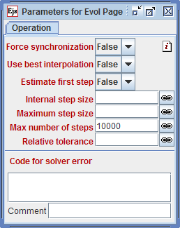
The Force synchonization option in the Advanced dialog can help you force a synchronization after every evolution step. This is usually overkill and is therefore false by default. You should only resort to this option when you suspect that the simulation is not producing correct values. If setting it to true makes your model work properly, then you most likely need a call to _resetSolvers() somewhere. Locate the problem, fix it, and set the Force synchonization parameter back to false.
Other advanced parameters
The advanced dialog offers two other parameters.
- The Estimate first step option is used by adaptive solvers to make an educated guess of an appropriated step size the very first time you step the evolution and after the solver is reset (by
_resetSolvers(), for instance). If the Estimate first step parameter is false, the Internal step field or (if this field is empty) the reading step is used instead. If the initial step size step is too large, the adaptive solver will unnecessarily spend a number of initial attempts to reach the prescribed tolerance. In normal situations, the reading step is a reasonable first attempt which is the reason why the parameter is false by default.
- The Internal step size is used both by adaptive and fixed-step solvers, if only differently.
- Adaptive solvers use it, as indicated above, as the value of an initial step if the Estimate first step parameter is
false.
- Fixed step solvers can use this parameter to indicate the solver to use an internal step different of the reading step. This possibility is seldom used, but you could use it, for example, to step a fixed step method at 0.001 while reading the solution at 0.1. This selection increases the precision of the solution, while reducing the number of output states. The result is a simulation that runs faster and with a high precision. The simulation runs faster because number-crunching is usually much faster than the visualization routines. (Note that setting the SPD value to 100 and a reading step of 0.001 produces a similar increase in speed, but will produce 100 more points in a plot of the solution.)